A First Glimpse of Rigetti’s Quantum Computing Cloud

Quantum computing has been picking up the momentum, and there are many startups and scholars discussing quantum machine learning. A basic knowledge of quantum two-level computation ought to be acquired.

Recently, Rigetti, a startup for quantum computing service in Bay Area, published that they opened to public their cloud server for users to simulate the use of quantum instruction language, as described in their blog and their White Paper. It is free.

Go to their homepage, http://rigetti.com/, click on “Get Started,” and fill in your information and e-mail. Then you will be e-mailed keys of your cloud account. Copy the information to a file .pyquil_config, and in your .bash_profile, add a line

export PYQUIL_CONFIG="$HOME/.pyquil_config"

More information can be found in their Installation tutorial. Then install the Python package pyquil, by typing in the command line:

pip install -U pyquil

Some of you may need to root (adding sudo in front).

Then we can go ahead to open Python, or iPython, or Jupyter notebook, to play with it. For the time being, let me play with creating an entangled singlet state, 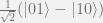. The corresponding quantum circuit is like this:

First of all, import all necessary libraries:

import numpy as np

from pyquil.quil import Program
import pyquil.api as api
from pyquil.gates import H, X, Z, CNOT

You can see that the package includes a lot of quantum gates. First, we need to instantiate a quantum simulator:

# starting the quantum simulator
quantum_simulator = api.SyncConnection()

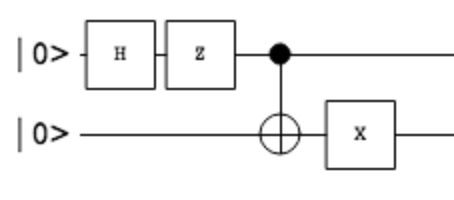
Then we implement the quantum circuit with a “program” as follow:

# generating singlet state
# 1. Hadamard gate
# 2. Pauli-Z
# 3. CNOT
# 4. NOT
p = Program(H(0), Z(0), CNOT(0, 1), X(1))
wavefunc, _ = quantum_simulator.wavefunction(p)

The last line gives the final wavefunction after running the quantum circuit, or “program.” For the ket, the rightmost qubit is qubit 0, and the left of it is qubit 1, and so on. Therefore, in the first line of the program, H, the Hadamard gate, acts on qubit 0, i.e., the rightmost qubit. Running a simple print statement:

print wavefunc

gives

(-0.7071067812+0j)|01> + (0.7071067812+0j)|10>

The coefficients are complex, and the imaginary part is described by j. You can extract it as a numpy array:

wavefunc.amplitudes

If we want to calculate the metric of entanglement, we can use the Python package pyqentangle, which can be installed by running on the console:

pip install -U pyqentangle

Import them:

from pyqentangle import schmidt_decomposition
from pyqentangle.schmidt import bipartitepurestate_reduceddensitymatrix
from pyqentangle.metrics import entanglement_entropy, negativity

Because pyqentangle does not recognize the coefficients in the same way as pyquil, but see each element as the coefficients of , we need to reshape the final state first, by:

tensorcomp = wavefunc.amplitudes.reshape((2, 2))

Then perform Schmidt decomposition (which the Schmidt modes are actually trivial in this example):

# Schmidt decomposition
schmidt_modes = schmidt_decomposition(tensorcomp)
for prob, modeA, modeB in schmidt_modes:
   print prob, ' : ', modeA, ' ', modeB

This outputs:

0.5  :  [ 0.+0.j  1.+0.j]   [ 1.+0.j  0.+0.j]
0.5  :  [-1.+0.j  0.+0.j]   [ 0.+0.j  1.+0.j]

Calculate the entanglement entropy and negativity from its reduced density matrix:

print 'Entanglement entropy = ', entanglement_entropy(bipartitepurestate_reduceddensitymatrix(tensorcomp, 0))
print 'Negativity = ', negativity(bipartitepurestate_reduceddensitymatrix(tensorcomp, 0))

which prints:

Entanglement entropy =  0.69314718056
Negativity =  -1.11022302463e-16

The calculation can be found in this thesis.

P.S.: The circuit was drawn by using the tool in this website, introduced by the Marco Cezero’s blog post. The corresponding json for the circuit is:

{"gate":[],{"gate":[], "circuit": [{"type":"h", "time":0, "targets":[0], "controls":[]},     {"type":"z", "time":1, "targets":[0], "controls":[]},     {"type":"x", "time":2, "targets":[1], "controls":[0]},     {"type":"x", "time":3, "targets":[1], "controls":[]}], "qubits":2,"input":[0,0]}
  

Release of shorttext 0.5.4

The Python package for text mining shorttext has a new release: 0.5.4. It can be installed by typing in the command line:

pip install -U shorttext

For some people, you may need to install it from “root”, i.e., adding sudo in front of the command. Since the version 0.5 (including releases 0.5.1 and 0.5.4), there have been substantial addition of functionality, mostly about comparisons between short phrases without running a supervised or unsupervised machine learning algorithm, but calculating the “similarity” with various metrics, including:

• soft Jaccard score (the same kind of fuzzy scores based on edit distance in SOCcer),
• Word Mover’s distance (WMD, detailedly described in a previous post), and
• Jaccard index due to word-embedding model.

For the soft Jaccard score due to edit distance, we can call it by:

>>> from shorttext.metrics.dynprog import soft_jaccard_score
>>> soft_jaccard_score(['book', 'seller'], ['blok', 'sellers'])     # gives 0.6716417910447762
>>> soft_jaccard_score(['police', 'station'], ['policeman'])        # gives 0.2857142857142858

The core of this code was written in C, and interfaced to Python using SWIG.

For the Word Mover’s Distance (WMD), while the source codes are the same as my previous post, it can now be called directly. First, load the modules and the word-embedding model:

>>> from shorttext.metrics.wasserstein import word_mover_distance
>>> from shorttext.utils import load_word2vec_model
>>> wvmodel = load_word2vec_model('/path/to/model_file.bin')

And compute the WMD with a single function:

>>> word_mover_distance(['police', 'station'], ['policeman'], wvmodel)                      # gives 3.060708999633789
>>> word_mover_distance(['physician', 'assistant'], ['doctor', 'assistants'], wvmodel)      # gives 2.276337146759033

And the Jaccard index due to cosine distance in Word-embedding model can be called like this:

>>> from shorttext.metrics.embedfuzzy import jaccardscore_sents
>>> jaccardscore_sents('doctor', 'physician', wvmodel)   # gives 0.6401538990056869
>>> jaccardscore_sents('chief executive', 'computer cluster', wvmodel)   # gives 0.0022515450768836143
>>> jaccardscore_sents('topological data', 'data of topology', wvmodel)   # gives 0.67588977344632573

Most new functions can be found in this tutorial.

And there are some minor bugs fixed.