Tensor Networks in Machine Learning: Part I

In 2019, Google published a new Python library called “tensornetwork” (arXiv:1905.01330) that facilitates the computation of… tensor networks. Tensor network is a tool from quantum many-body theory, widely used in condensed matter physics. There have been a lot of numerical packages for tensor computation, but this library takes it to the next level because of its distinctive framework.

What is a tensor network, though?

“A tensor network is a collection of tensors with indices connected according to a network pattern. It can be used to efficiently represent a many-body wave-function in an otherwise exponentially large Hilbert space.”

https://www.perimeterinstitute.ca/research/research-initiatives/tensor-networks-initiative

Renormalization Group (RG)

It is not until recently that tensor networks have its application in machine learning. As stated in a previous post, a mathematical connection between restricted Boltzmann machine (RBM) and variational renormalization group (RG) was drawn. (arXiv:1410.1831) It shedded light to the understanding of interpretability of deep learning, which has been criticized to be a black box. However, RBM is just a type of unsupervised machine learning, but how about others?

Seeing this, Schwab, one of the authors of the RG paper, and Stoudenmire did some work to realize the use of RG in machine learning. Stoudenmore is a physicist, and he made use of density matrix renormalization group (DMRG) that he is familiar with, and invented a supervised learning algorithm, which is later renamed tensor network machine learning (TNML). The training is adapted from the sweeping algorithm, the standard of DMRG, that combining bipartite site one-by-one, updating it, and decomposing into two site by studying its quantum entanglment (using singular value decomposition, or Schmidt decomposition).

Instead of bringing interpretability to deep learning, this work in fact opened a new path of new machine learning algorithms with known techniques.

What is RG?

Renormalization group (RG) is a formalism of “zooming out” in scale-invariant system, determining which terms to truncate in a model. It is an important formalism in high energy physics and statistical field theory. (See Ma’s book for reference.)

Density matrix renormalization group (RG) is a variational real-space numerical technique that look at collections of quantum bits (zoomed-out) as a block. It was invented by Steven White, and it is useful in studying strongly correlated electronic systems. (PRL 69 (19): 2863-2866 (1992)). However, the original DMRG paper is not very accessible, until it is rephrased using the tensor network notation (TNN), as shown in Schollwoeck’s article.

Is Tensor Network Related to Quantum Computing?

This is not an easy question to answer. Tensor networks come from quantum physics, but quantum physics is usually not directly leading to quantum computing. In fact, classical computing hardwares have a lot of quantum physics in it. A simple answer to this question is no, as the algorithm using tensor network is implemented in classical computers.

There have been a lot of publications on quantum machine learning lately. A classic book on this topic is written by Peter Wittek. The book covers topics on basic machine learning and quantum computing, and then quantum machine learning algorithms. There is a quantum counterpart of each of the common machine learning algorithms in the book. However, we know it would be much more useful if there are new algorithms exploiting the advantages of quantum computing. Tensor network is a natural choice as it builds on qubits, and the representations and operations are naturally quantum.

Next…

Tensor network is an interesting subject from both a theoretical and applicational perspective. In coming posts I will talk about its application on machine learning and a taste of codes.

---

• Github: google/TensorNetwork. [Github] [RTFD]
• Chase Roberts, Ashley Milsted, Martin Ganahl, Adam Zalcman, Bruce Fontaine, Yijian Zou, Jack Hidary, Guifre Vidal, Stefan Leichenauer, “TensorNetwork: A Library for Physics and Machine Learning,” arXiv:1905.01330 (2019). [arXiv]
• “Google TensorNetwork Library Dramatically Accelerates ML & Physics Tasks,” Syncedreview. (2019) [Medium]
• Chase Roberts, “Introducing TensorNetwork, an Open Source Library for Efficient Tensor Calculations,” Google AI Blog. (2019) [GoogleAIBlog]
• “Tensor Networks and Density Matrix Renormalization Group,” Everything About Data Analytics. (2016) [WordPress]
• P. Mehta, D. J. Schwab, “An exact mapping between the Variational Renormalization Group and Deep Learning,” arXiv:1410.3831 (2014). [arXiv]
• Sheng-kang Ma, Modern Theory of Critical Phenomena, (New York, NY: Routledge, 2018). [Amazon]
• S. R. White, “Density matrix formulation for quantum renormalization groups,” Phys. Rev. Lett. 69, 2863 (1992). [APS]
• Ulrich Schollwoeck, “The density-matrix renormalization group,” Rev. Mod. Phys. 77, 259 (2005); arXiv:cond-mat/0409292. [arXiv]
• Ulrich Schollwoeck, “The density-matrix renormalization group in the age of matrix product states,” Annals of Physics 326, 96 (2011); arXiv:1008.3477. [arXiv]
• Peter Wittek, Quantum Machine Learning: What Quantum Computing Means to Data Mining (San Diego, CA: Academic Press, 2014). [Amazon] [PDF]
• Jacob Biamonte, Peter Wittek, Nicola Pancotti, Patrick Rebentrost, Nathan Wiebe, Seth Lloyd, “Quantum Machine Learning,” Nature 549, 195-202 (2017). [Nature]
• Tensor Networks: From Entangled Quantum Matter to Emergent Space Time, Perimeter Institute. [Perimeter]

Feature picture taken from Perimeter Institute.

Data Representation in Machine Learning

In implementing most of the machine learning algorithms, we represent each data point with a feature vector as the input. A vector is basically an array of numerics, or in physics, an object with magnitude and direction. How do we represent our business data in terms of a vector?

Primitive Feature Vector

Whether the data are measured observations, or images (pixels), free text, factors, or shapes, they can be categorized into four following types:

1. Categorical data
2. Binary data
3. Numerical data
4. Graphical data

The most primitive representation of a feature vector looks like this:

A typical feature vector. (Source: https://www.researchgate.net/publication/318740904_Chat_Detection_in_an_Intelligent_Assistant_Combining_Task-oriented_and_Non-task-oriented_Spoken_Dialogue_Systems/figures?lo=1)

Numerical Data

Numerical data can be represented as individual elements above (like Tweet GRU, Query GRU), and I am not going to talk too much about it.

Categorical Data

However, for categorical data, how do we represent them? The first basic way is to use one-hot encoding:

One-hot encoding of categorical data (Source: https://developers.google.com/machine-learning/data-prep/transform/transform-categorical)

For each type of categorical data, each category has an integer code. In the figure above, each color has a code (0 for red, 1 for orange etc.) and they will eventually be transformed to the feature vector on the right, with vector length being the total number of categories found in the data, and the element will be filled with 1 if it is of that category. This allows a natural way of dealing with missing data (with all elements 0) and multi-category (with multiple non-zeros).

In natural language processing, the bag-of-words model is often used to represent free-text data, which is the one-hot encoding above with words as the categories. It is a good way as long as the order of the words does not matter.

Binary Data

For binary data, it can be easily represented by one element, either 1 or 0.

Graphical Data

Graphical data are best represented in terms of graph Laplacian and adjacency matrix. Refer to a previous blog article for more information.

Shortcomings

A feature vector can be a concatenation of various features in terms of all these types except graphical data.

However, such representation that concatenates all the categorical, binary, and numerical fields has a lot of shortcomings:

1. Data with different categories are often seen as orthogonal, i.e., perfectly dissimilar.  It ignores the correlation between different variables. However, it is a very big assumption.
2. The weights of different fields are not considered.
3. Sometimes if the numerical values are very large, it outweighs other categorical data in terms of influence in computation.
4. Data are very sparse, costing a lot of memory waste and computing time.
5. It is unknown whether some of the data are irrelevant.

Modifying Feature Vectors

In light of the shortcomings, to modify the feature factors, there are three main ways of dealing with this:

1. Rescaling: rescaling all of some of the elements, or reweighing, to adjust the influence from different variables.
2. Embedding: condensing the information into vectors of smaller lengths.
3. Sparse coding: deliberately extend the vectors to a larger length.

Rescaling

Rescaling means rescaling all or some of the elements in the vectors. Usually there are two ways:

1. Normalization: normalizing all the categories of one feature to having the sum of 1.
2. Term frequency-inverse document frequency (tf-idf): weighing the elements so that the weights are heavier if the frequency is higher and it appears in relatively few documents or class labels.

Embedding

Embedding means condensing a sparse vector to a smaller vector. Many sparse elements disappear and information is encoded inside the elements. There are rich amount of work on this.

1. Topic models: finding the topic models (latent Dirichlet allocation (LDA),  structural topic models (STM) etc.) and encode the vectors with topics instead;
2. Global dimensionality reduction algorithms: reducing the dimensions by retaining the principal components of the vectors of all the data, e.g., principal component analysis (PCA), independent component analysis (ICA), multi-dimensional scaling (MDS) etc;
3. Local dimensionality reduction algorithms: same as the global, but these are good for finding local patterns, where examples include t-Distributed Stochastic Neighbor Embedding (tSNE) and Uniform Manifold Approximation and Projection (UMAP);
4. Representation learned from deep neural networks: embeddings learned from encoding using neural networks, such as auto-encoders, Word2Vec, FastText, BERT etc.
5. Mixture Models: Gaussian mixture models (GMM), Dirichlet multinomial mixture (DMM) etc.
6. Others: Tensor decomposition (Schmidt decomposition, Jennrich algorithm etc.), GloVe etc.

Sparse Coding

Sparse coding is good for finding basis vectors for dense vectors.

Discriminative Adversarial Networks

Generative adversarial networks (GANs) have made a big impact to the world of machine learning. It is particularly useful for generating sample data when there are insufficient data for certain purposes. It is also useful for training using data with both labeled and unlabeled data, i. e., semi-supervised learning. (SSL)

The rise of GANs also lead to the re-emergence of adversarial learning regarding the handling of unbalanced data or sensitive data. (For example, see arXiv:1707.00075.)

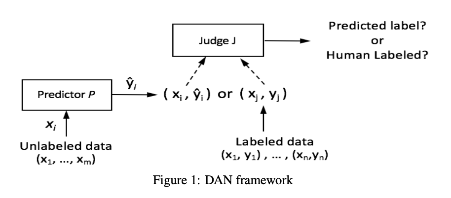
GAN is particularly useful for computer vision problems. However, it is not very good for natural language problems as the data cannot be generated continuously. Under this context, a modification on GAN is developed, called discriminative adversarial networks (DAN, see arXiv:1707.02198.). Unlike GANs that has a discriminator to train a generator to produce good data, DAN has two discriminators: one discriminator, usually denoted as the predictor P, that predicts on the unlabeled data, and another, usually denoted as the judge J, that classifies whether the label is a human label or a machine-predicted label.

The loss function of DAN is very similar to that of GAN: minimizing the entropy difference for the judge J for labeled data, but minimizing that for predictions for unlabeled data for the predictor P.

However, GAN and DAN are not generative-disciminative pairs.

Strategies of Recommendation Systems

Systems developed by enterprises such as Netflix produce recommendations. Good recommendations induce good user experience and higher return rates. Humans give recommendations based on experience, knowledge, worldviews, wisdom etc., and automatic recommendation systems do it based on big data and machine learning.

Recommendation Strategies

Recommendation systems employ one or more of the following strategies:

1. Collaborative Filtering (CF);
2. Content-based Filtering (CBF);
3. Demographic Filtering (DF); and
4. Knowledge-Based Filtering (KBF).

1. Collaborative Filtering (CF)

CF recommends similar items to users of similar tastes. Whether it is user-based filtering or item-based filtering, the same assumption holds. Similarity between users or items are calculated by Pearson correlations or cosine similarities.

Matrix Factorization (MF), or similar latent semantic indexing (LSI) is actually a kind of collaborative filtering, although the users or items are converted to an encoded vector, and the recommendation scores are given by the cosine similarity between the encoded vectors of the users and the items.

Such recommendation systems suffer the cold-start problem: new users or new items cannot be accounted for when giving recommendations.

2. Content-Based Filtering (CBF)

CBF employs common machine learning algorithms to learn a user’s preference based on their consumption/purchase history and their profiles. Embedded vectors will be used too. However, this suffer cold-start problem.

3. Demographic Filtering (DF)

DF strategy makes use of users’ profiles such as age, sex, and other information to make recommendations. The algorithms might be rule-based, or machine learning also. However, nowadays, it might give rise to issues regarding fairness, equal opportunities, privacy, or ethics, in the wake of the era of GDPR or CCPA.

4. Knowledge-Based Filtering (KBF)

KBF makes recommendations based on the expert knowledge of the subject matter, known reasoning, or statistics. Recommendations may be made using a rule-based approach, or a predefined probabilistic model (such as census data). Some might have even employ a knowledge database. Big data may not be necessary in this kind of systems as the reasoning has been manually built-in.

Hybrid Recommendation Systems

Hybrid recommendation systems employ more than one of the above strategies. To combine all these strategies, one might put a voting system to all the results to give an aggregated results, or a weighting scheme, or a stacked generalization to combine all these methods together.

Mathematical Models of Fake News

Fake news is not something new, but it catches our attention since the 2016 presidential election campaign. Some people label a piece of news fake news if it does not align with its ideological elements in its analysis. Fake news are necessarily biased, although truth are inevitably not neutral as well. While a lot of technological tycoons want to handle fake news appropriately in their platform, a lack of a formal definition makes it difficult.

It has been introduced in previous entry that in order to detect fake news using machine learning, we have to provide a corpus. This provides a paveway to train supervised learning models.

Recently, some people look at this problem in a different way from the sociological point of view. In order to evaluate the impact imposed by fake news, instead of having a machine learning model, we need a dynamical model of the spread of fake news. In their preprint in arXiv, Brody and Meier studied it using the tools in communication theory. They proposed that the flow of information is:

,

where is time, is either 0 or 1 indicating the news is false or true respectively, is noise (Brownian motion), and is the fake news. The first term indicates that we have more information over time, and thus the flow of true information increases with time. This model assumes a linear evolution. The authors define to be fake news if its expection $latex \mathop{\mathbb{E}} (F_t) \neq 0$. Depending on the situation, and are either independent or correlated.

To study the impact, the authors categorized voters into three categories:

• Category I: unaware of the existence of fake news, but act rationally;
• Category II: aware of the existence of fake news, but unaware of the time point when fake news emerges;
• Category III: fully aware of the existence of fake news, and fully eliminated them when making a judgement.

There are further mathematical models to model the election dynamics, but readers can refer the details to the preprint. With a piece of fake news in favor of candidate B, this model gives the influence of fake news on one’s judgment, as plotted below:

This dynamical model confirms that by eliminating the fake news, the voters make better judgment. However, with the awareness of the piece of fake news emerging at a time unknown to the voter, the impact is still disastrous.

To me, this study actually confirms that the fact check is useless in terms or curbing the turmoil introduced by fake news. The flow of information nowadays is so without viscosity that ways to eliminate fake news has to be derived. However, we know censorship is not the way to go as it is a highway to a totalitarian government. The future of democracy is dim.

Use of Graph Networks in Machine Learning

Deep learning has achieved a big success in the past few years, but its interpretive power is limited. They work largely because of the abundance of data. On the other hand, traditional machine learning algorithms are much better in interpretive power, but manual feature engineering costs a lot, due to the lack of data in earlier era. In light of this, a group of scientists initiated the work of graph networks, aiming at devising new artificial intelligence algorithms that exploits the advantages of two worlds, while still holding the principle of combinatorial generalization in constructing methods by using known building blocks to build new methods. Graph is good at interpretation as it is good for relational representation.

The use of graph networks is more than the graph convolutional neural networks (GCN) in the previous two blog entries. (part I and part II) However, to achieve relational inductive biases, an entity (an element with attributes), a relation, (a property between entities) and a rule. (a function that maps entities and relations to other entities and relations) This can be realized using graph, which is a mathematical structure that contains nodes and edges (that connect nodes.) To generalize the use of graph networks in various machine learning and deep learning methods, they reviewed the graph block, which is basically a function, or a mapping, from a graph to another graph, as shown in the algorithm below:

Works of graph networks are not non-existent; the authors listed previous works that can be seen as graph networks, for example:

• Message-passing neural network (MPNN) (2017);
• Non-local neural networks (NLNN) (2018).

The use of graph networks, I believe, is the next trend. There have been works regarding the graph-powered machine learning. (see Google AI blog, GraphAware Slideshare) I recently started an open-source project, a Python package called graphflow, to explore various algorithms using graphs, including PageRank, HITS, resistance, and non-linear resistance.

Graph Convolutional Neural Network (Part II)

In the previous post, the convolution of the graph Laplacian is defined in its graph Fourier space as outlined in the paper of Bruna et. al. (arXiv:1312.6203) However, the eigenmodes of the graph Laplacian are not ideal because it makes the bases to be graph-dependent. A lot of works were done in order to solve this problem, with the help of various special functions to express the filter functions. Examples include Chebyshev polynomials and Cayley transform.

ChebNet

Kipf and Welling proposed the ChebNet (arXiv:1609.02907) to approximate the filter using Chebyshev polynomial, using the result proved by Hammond et. al. (arXiv:0912.3848) With a convolutional layer , instead of computing it directly by , it approximates the filter in terms of Chebyshev polynomial:

,

where are the Chebyshev polynomials. It has been proved by Hammond et. al. that by well truncating this representation, Chebyshev polynomials are very good to approximate the function. Then the convolution is:

.

Here, ’s are the parameters to be trained. This fixed the bases of the representation, and it speeds up computation. The disadvantage is that eigenvalues are clusters in a few values with large gaps.

CayleyNet

The problem of ChebNet led to the work of Levie et. al., (arXiv:1705.07664) who proposed another approximation is used using Cayley transform. They made use of the Cayley function:

,

which is a bijective function from to complex unit half-circle. Instead of Chebyshev polynomials, it approximates the filter as:

,

where is real and other ’s are generally complex, and is a zoom parameter, and ’s are the eigenvalues of the graph Laplacian. Tuning $h$ makes one find the best zoom that spread the top eigenvalues. ‘s are computed by training. This solves the problem of unfavorable clusters in ChebNet.

MotifNet

All previous works are undirected graph. How do we deal with directed graph with an asymmetric graph Laplacian? Benson, Gleich, Leskovec published an important work on Science in 2016 (arXiv:1612.08447) to address this problem. Their approach is reducing a directed graph to a higher order structure called network motifs. There are 13 network motifs. For each network motif, one can define an adjacency matrix for that motif by , with elements being the number of motifs in the graph the the edge that it belongs to.

Then one computes 13 graph Laplacians from these 13 adjacency matrices. These graph Laplacians are symmetric, like those of undirected graphs. Then any filters can be approximated by the following multivariate matrix polynomial, as suggested by Monti, Otness, and Bronstein in their MotifNet paper (arXiv:1802.01572):

.

Applications of image processing, citation networks etc.

Graph Convolutional Neural Network (Part I)

Suggested by some friends, I have been reading graph convolutional neural network. This is not a recent interest, as I have been interested in some graph-related problems (as I developed the graphflow package) and topological data analysis (TDA, as I developed the mogutda package). Graph theory is not a new field as well, but it is interesting to see how it is being applied in deep learning, as a lot of real-world relational data can be expressed in terms of graphs. (Examples: word relations, organizational structure, genes, internet etc.) With the increasing attention to neo4j, we know graph is coming to be hot.

It would be helpful to review some basic graph theory:

• A graph is represented by , where and are the nodes (vertices) and edges respectively.
• A graph can be directed or undirected. In graph convolutional neural network, they are undirected usually.
• The adjacency matrix describes how nodes are connected: if there is an edge connecting from node to node , and otherwise. is a symmetric matrix for an undirected graph.
• The incidence matrix is another way to describe how nodes are connected: if a node is connected with edge . This is useful for undirected graph.
• The degree matrix is a diagonal matrix, with elements denotes the number of neighbors for node in undirected matrix.
• The function acting on the nodes is called the filter.
• The graph Laplacian, or Kirchhoff matrix, is defined by , and the normalized graph Laplacian is .

The graph Laplacian is the most important matrix in graph convolutional neural network. It is analogous to the Laplacian operator in Euclidean space, . The reader can easily verify this by constructing a graph of 2D lattice and compute the graph Laplacian matrix, and find that it is the same as the discretized Laplacian operator.

We can also get some insights from the Euclidean analogue. In physics, the solution to the Laplacian equation is harmonic: the basis of the solution can be described in the spectral/Fourier space, as:

,

And . In graph convolutional neural network, as Bruna et. al. suggested in 2013, the graph is calculated in the graph Fourier space, instead of directly dealing with the Laplacian matrix in all layers of network.

On the other hand, we know that for the convolution

,

its Fourier transform is given by

.

In Fourier space, the convolution of two functions are just their products. Similarly, in graph convolutional neural network, convolutions can be computed in the Fourier space as the mere product of two filters in the Fourier space. More specifically, for finding the convolution of the filters and , with being the unitary eigenmatrix,

.

However, such general description is basis-dependent, and it is still computationally expensive. More work has been proposed to smooth the representation, which will be covered in the upcoming blogs.

A side note, the readers can verify themselves that

Embedded Language Models

Sebastian Ruder recently wrote an article on The Gradient and asserted that the oracle of natural language processing is emerging. While I am not sure such confident statement is overstated, I do look forward to the moment that we will download pre-trained embedded language models and transfer to our use cases, just like we are using pre-trained word-embedding models such as Word2Vec and FastText.

I do not think one can really draw a parallelism between computer vision and natural language processing. Computer vision is challenging, but natural language processing is even more difficult because the tasks regarding linguistics are not limited to object or meaning recognition, but also human psychology, cultures, and linguistic diversities. The objectives are far from being identical.

However, the transferrable use of embedded language models is definitely a big step forward. Ruder quoted three articles, which I would summarize below in a few words.

• Embeddings from Language Models (ELMo, arXiv:1802.05365): based on the successful bidirectional LSTM language models, the authors developed a deep contextualized embedded models by collapses all layers in the neural network architecture.
• Universal Language Model Fine-Tuning for Text Classification (ULMFiT, arXiv:1801.06146): the authors proposed a type of architectures that learn representations for specific tasks, which involve three steps in training: a) LM pre-training: learning through unlabeled corpus with abundant data; b) LM fine-tuning: learning through labeled corpus; and c) classifier fine-tuning: transferred training for specific classification tasks.
• OpenAI Transformer (article still in progress): the author proposed a simple generative language model with the three similar steps in ULMFit: a) unsupervised pre-training: training a language model that maximizes the likelihood of a sequence of tokens within a context window; b) supervised fine-tuning: a supervised classification training that maximizes the likelihood using the Bayesian approach; c) task-specific input transformations: training the classifiers on a specific task.

These three articles are intricately related to each other. Without abundant data and good hardware, it is almost impossible to produce the language models. As Ruder suggested, we will probably have a pre-trained model up to the second step of the ULMFit and OpenAI Transformer papers, but we train our own specific model for our use. We have been doing this for word-embedding models, and this approach has been common in computer vision too.

moguTDA: Python package for Simplicial Complex

It has been a while since I wrote about topological data analysis (TDA). For pedagogical reasons, a lot of the codes were demonstrated in the Github repository PyTDA. However, it is not modularized as a package, and those codes run in Python 2.7 only.

Upon a few inquiries, I decided to release the codes as a PyPI package, and I named it mogutda, under the MIT license. It is open-source, and the codes can be found at the Github repository MoguTDA. It runs in Python 2.7, 3.5, and 3.6.

For more information and simple tutorial, please refer to the documentation, or the Github page.