Leo Kadanoff is an American physicist in University of Chicago. His most prominent work is the idea of block spin and coarse-graining in statistical physics. [Kadanoff 1966] His work has an enormous impact on second-order phase transition and critical phenomena, based on the knowledge of scale and universality. His idea was further developed into renormalization group (RG), [Wilson 1983] which leads to Ken Wilson awarded with Nobel Prize in Physics in 1982.
The concept of RG has also been used to explain how deep learning works, [Mehta, Schwab 2014] which you can read more about from my previous blog entry and their paper. While only the equivalence between RG and Restricted Boltzmann Machine was rigorously proved, it sheds a lot of insights about how it works, in a way that I believe it is roughly what happens. Without the concept that Kadanoff developed, it is impossible for Mehta and Schwab to make such a connection between critical phenomena and neural network.
He has other contributions such as computational physics, urban planning, computer science, hydrodynamics, biology, applied mathematics and geophysics. He has been awarded with the Wolf Prize in Physics (1980), Elliott Cresson Medal(1986), Lars Onsager Prize (1998), Lorentz Medal (2006), and Isaac Newton Medal (2011).
His work has a significant impact on statistical physics, including problems of second-order phase transition, percolation, various condensed matter systems (such as conventional superconductors, superfluids, low-dimensional systems, helimagnets), quantum phase transition, self-organized criticality etc. To learn more about it, I highly recommend Shang-keng Ma’s Modern Theory of Critical Phenomena [Ma 1976] and Mehran Karder’s Statistical Physics of Fields. [Karder 2007]
Rest In Peace!
Leo Kadanoff (1937-2015) (taken from the homepage of University of Chicago)
One fascinating application of deep learning is the training of a model that outputs vectors representing words. A project written in Google, named Word2Vec, is one of the best tools regarding this. The vector representation captures the word contexts and relationships among words. This tool has been changing the landscape of natural language processing (NLP).
Let’s have some demonstration. To use Word2Vec in Python, you need to have the package gensim installed. (Installation instruction: here) And you have to download a trained model (GoogleNews-vectors-negative300.bin.gz), which is 3.6 GB big!! When you get into a Python shell (e.g., IPython), type
from gensim.models.word2vec import Word2Vec
model = Word2Vec.load_word2vec_format('GoogleNews-vectors-negative300.bin', binary=True)
This model enables the user to extract vector representation of length 300 of an English word. So what is so special about this vector representation from the traditional bag-of-words representation? First, the representation is standard. Once trained, we can use it in future training or testing dataset. Second, it captures the context of the word in a way that the algebraic operation of these vectors has meanings.
Here I give 5 examples.
A Juvenile Cat
What is a juvenile cat? We know that a juvenile dog is a puppy. Then we can get it by carry out the algebraic calculation by running
which indicates that “kitten” is the answer (correctly!) The numbers are similarities of these words with the vector representation in descending order. You can verify it by calculating the cosine distance:
from scipy.spatial import distance
print (1-distance.cosine(model['kitten'], model['puppy']+model['cat']-model['dog']))
which outputs 0.763498957413.
Mogu, my cat, three years ago when she was still a kitten
This demonstration shows that in the model, and are of similar semantic relations.
Capital of Taiwan
Where is the capital of Taiwan? We can find it if we know the capital of another country. For example, we know that Beijing is the capital of China. Then we can run the following:
However, this model does not always work. If it can find the capital of Taiwan, can it find those for any states in the United States? We know that the capital of California is Sacramento. How about Maryland? Let’s run:
Blue crabs (lunch in Cantler’s Riverside Inn, Annapolis, MD)
More About Word2Vec
Word2Vec was developed by Tomáš Mikolov. He previously worked for Microsoft Research. However, he switched to Google, and published a few influential works on Word2Vec. [Mikolov, Yih, Zweig 2013] [Mikolov, Sutskever, Chen, Corrado, Dean 2013] [Mikolov, Chen, Corrado, Dean 2013] Their conference paper in 2013 can be found on arXiv. He later published a follow-up work on a package called Doc2Vec that considers phrases. [Le, Mikolov 2014]
Earlier this year, I listened to a talk in DCNLP meetup spoken by Michael Czerny on his award-winning blog entry titled “Modern Methods for Sentiment Analysis.” He applied the vector representations of words by Word2Vec to perform sentiment analysis, assuming that similar sentiments cluster together in the vector space. (He took averages of the vectors in tweets to extract emotions.) [Czerny 2015] I highly recommend you to read his blog entry. On the other hand, Xin Rong wrote an explanation about how Word2Vec works too. [Rong 2014]
There seems to be no progress on the project Word2Vec anymore as Tomáš Mikolov no longer works in Google. However, the Stanford NLP Group recognized that Word2Vec captures the relations between words in their vector representation. They worked on a similar project, called GloVe (Global Vectors), which tackles the problem with matrix factorization. [Pennington, Socher, Manning 2014] Radim Řehůřek did some analysis comparing Word2Vec and GloVe. [Řehůřek 2014] GloVe can be implemented in Python too.
On October 14, 2015, I attended the regular meeting of the DCNLP meetup group, a group on natural language processing (NLP) in Washington, DC area. The talk was titled “Deep Learning for Question Answering“, spoken by Mr. Mohit Iyyer, a Ph.D. student in Department of Computer Science, University of Maryland (my alma mater!). He is a very good speaker.
I have no experience on deep learning at all although I did write a blog post remotely related. I even didn’t start training my first neural network until the next day after the talk. However, Mr. Iyyer explained what recurrent neural network (RNN), recursive neural network, and deep averaging network (DAN) are. This helped me a lot in order to understanding more about the principles of the famous word2vec model (which is something I am going to write about soon!). You can refer to his slides for more details. There are really a lot of talents in College Park, like another expert, Joe Yue Hei Ng, who is exploiting deep learning a lot as well.
The applications are awesome: with external knowledge to factual question answering, reasoning-based question answering, and visual question answering, with increasing order of challenging levels.
Mr. Iyyer and the participants discussed a lot about different packages. Mr. Iyyer uses Theano, a Python package for deep learning, which is good for model building and other analytical work. Some prefer Caffe. Some people, who are Java developers, also use deeplearning4j.
Stetsons Famous Bar & Grill (photo from Yelp)
This meetup was a sacred one too, because it is the last time it was held in Stetsons Famous Bar & Grill at U Street, which is going to permanently close on Halloween this year. The group is eagerly looking for a new venue for the upcoming meetup. This meeting was a crowded one. I sincerely thank the organizers, Charlie Greenbacker and Liz Merkhofer, for hosting all these meetings, and Chris Phipps (a linguist from IBM Watson) for recording.
There is no doubt that everyone who are in the so-called big data industry must know some statistics. However, statistics means differently to different peoples.
Traditional Statistics
Statistics is an old field that was developed in the 18th century. In those times, people were urged to make conclusions out of a vast amount of data which were virtually not available, or were very costly to obtain. For example, someone wanted to know the average salary of the whole population, which required the census staff to survey the information from everyone in the population. It was something expensive to do in the old days. Therefore, sampling techniques were devised, and the wanted quantities can be estimated using an appropriate statistic.
Or when the scientists performed an experiment, even one data point costs a few million dollars. The experiments had to be designed in a way that the scientists extract the wanted information by looking at a few data points.
Or in testing some hypotheses, one needs to know only how to accept or reject a hypothesis using the statistical information available.
Hence, the traditional statistics is a body of knowledge that deduce the information of a whole population from a limited amount of data from a sample.
Theoretical Statistical Physics
There is a branch in physics called statistical physics, which originated from the 19th century. Later it became useful since Albert Einstein published its paper on Brownian motion in 1905. And now the methods in statistical physics is not only applied in solid state physics or condensed matter physics, but also in biophysics (e.g., diffusion), econophysics (e.g., the fairness and wealth distribution, see this previous blog post), and quantitative finance (e.g., binomial model, and its relation with Black-Scholes equation).
The techniques involved in statistical physics includes is the knowledge of probability theory and stochastic calculus (such as Ito calculus). Of course, it is how entropy, a concept from thermodynamics, entered probability theory and information theory. Extracted quantity are mostly expectation values and correlations, which are of interest to theorists.
This is very different from traditional statistics. When people know that I am a statistical physicist, they expect me to be familiar with t-test, which is not really the case. (Very often I have to look up every time I used them.)
Statistics in the Computing World
Unlike in traditional statistics or statistical physics, nowadays, we often get the statistical information directly from a vast amount of available data, thanks to the advance of technology and the reducing cost to access the technology. You can easily calculate the average salary of a population by a single command line on R or Python. Hence, statistics is no longer about extracting information from a limited amount of data, but a vast amount of data.
On the other hand, mathematical modeling is still important, but in a different sense. Models in statistical physics describes the world, but in information retrieval, models are built according to what we need.
P.S.: Philipp Janert wrote something similar in his Chapter 10 (“What You Really Need to Know About Classical Statistics”) in his “Data Analysis Using Open Source Tools“:
The basic statistical methods that we know today were developed in the late 19th and early 20th centuries, mostly in Great Britain, by a very small group of people. Of those, one worked for the Guinness brewing company and another—the most influential one of them—worked at an agricultural research lab (trying to increase crop yields and the like). This bit of historical context tells us something about their working conditions and primary challenges.
No computational capabilities All computations had to be performed with paper and pencil.
No graphing capabilities, either All graphs had to be generated with pencil, paper, and a ruler. (And complicated graphs—such as those requiring prior transformations or calculations using the data—were especially cumbersome.)
Very small and very expensive data sets Data sets were small (often not more than four to five points) and could be obtained only with great difficulty. (When it always takes a full growing season to generate a new data set, you try very hard to make do with the data you already have!)
In other words, their situation was almost entirely the opposite of our situation today:
Computational power that is essentially free (within reason)
Interactive graphing and visualization capabilities on every desktop
Often huge amounts of data
It should therefore come as no surprise that the methods developed by those early researchers seem so out of place to us: they spent a great amount of effort and ingenuity solving problems we simply no longer have! This realization goes a long way toward explaining why classical statistics is the way it is and why it often seems so strange to us today.
P.S.: The graph at the beginning of this blog entry was plotted in Mathematica, by running the following:


 by running
 and
and  are of similar semantic relations.
 Taipei (taken from Airasia:
 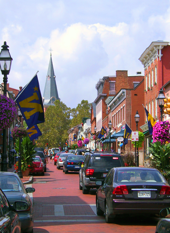 Downtown Annapolis (taken from Wikipedia)


