June 2017 – Everything about Data Analytics

Embedding algorithms, especially word-embedding algorithms, have been one of the recurrent themes of this blog. Word2Vec has been mentioned in a few entries (see this); LDA2Vec has been covered (see this); the mathematical principle of GloVe has been elaborated (see this); I haven’t even covered Facebook’s fasttext; and I have not explained the widely used t-SNE and Kohonen’s map (self-organizing map, SOM).

I have also described the algorithm of Sammon Embedding, (see this) which attempts to capture the likeliness of pairwise Euclidean distances, and I implemented it using Theano. This blog entry is about its implementation in Tensorflow as a demonstration.

Let’s recall the formalism of Sammon Embedding, as outlined in the previous entry:

Assume there are high dimensional data described by $d$ -dimensional vectors, $X_i$ where $i=1, 2, \ldots, N$ . And they will be mapped into vectors $Y_i$ , with dimensions 2 or 3. Denote the distances to be $d_{ij}^{*} = \sqrt{| X_i - X_j|^2}$ and $d_{ij} = \sqrt{| Y_i - Y_j|^2}$ . In this problem, $Y_i$ are the variables to be learned. The cost function to minimize is

$E = \frac{1}{c} \sum_{i<j} \frac{(d_{ij}^{*} - d_{ij})^2}{d_{ij}^{*}}$ ,

where $c = \sum_{i<j} d_{ij}^{*}$ .

Unlike in previous entry and original paper, I am going to optimize it using first-order gradient optimizer. If you are not familiar with Tensorflow, take a look at some online articles, for example, “Tensorflow demystified.” This demonstration can be found in this Jupyter Notebook in Github.

First of all, import all the libraries required:

import numpy as np
import matplotlib.pyplot as plt
import tensorflow as tf

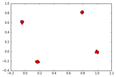
Like previously, we want to use the points clustered around at the four nodes of a tetrahedron as an illustration, which is expected to give equidistant clusters. We sample points around them, as shown:

tetrahedron_points = [np.array([0., 0., 0.]), np.array([1., 0., 0.]), np.array([np.cos(np.pi/3), np.sin(np.pi/3), 0.]), np.array([0.5, 0.5/np.sqrt(3), np.sqrt(2./3.)])]

sampled_points = np.concatenate([np.random.multivariate_normal(point, np.eye(3)*0.0001, 10) for point in tetrahedron_points])

init_points = np.concatenate([np.random.multivariate_normal(point[:2], np.eye(2)*0.0001, 10) for point in tetrahedron_points])

Retrieve the number of points, N, and the resulting dimension, d:

N = sampled_points.shape[0]
d = sampled_points.shape[1]

One of the most challenging technical difficulties is to calculate the pairwise distance. Inspired by this StackOverflow thread and Travis Hoppe’s entry on Thomson’s problem, we know it can be computed. Assuming Einstein’s convention of summation over repeated indices, given vectors $a_{ik}$ , the distance matrix is:

$D_{ij} = (a_{ik}-a_{jk}) (a_{ik} - a_{jk})^T = a_{ik} a_{ik} + a_{jk} a_{jk} - 2 a_{ik} a_{jk}$ ,

where the first and last terms are simply the norms of the vectors. After computing the matrix, we will flatten it to vectors, for technical reasons omitted to avoid gradient overflow:

X = tf.placeholder('float')
Xshape = tf.shape(X)

sqX = tf.reduce_sum(X*X, 1)
sqX = tf.reshape(sqX, [-1, 1])
sqDX = sqX - 2*tf.matmul(X, tf.transpose(X)) + tf.transpose(sqX)
sqDXarray = tf.stack([sqDX[i, j] for i in range(N) for j in range(i+1, N)])
DXarray = tf.sqrt(sqDXarray)

Y = tf.Variable(init_points, dtype='float')
sqY = tf.reduce_sum(Y*Y, 1)
sqY = tf.reshape(sqY, [-1, 1])
sqDY = sqY - 2*tf.matmul(Y, tf.transpose(Y)) + tf.transpose(sqY)
sqDYarray = tf.stack([sqDY[i, j] for i in range(N) for j in range(i+1, N)])
DYarray = tf.sqrt(sqDYarray)

And DXarray and DYarray are the vectorized pairwise distances. Then we defined the cost function according to the definition:

Z = tf.reduce_sum(DXarray)*0.5
numerator = tf.reduce_sum(tf.divide(tf.square(DXarray-DYarray), DXarray))*0.5
cost = tf.divide(numerator, Z)

As we said, we used first-order gradient optimizers. For unknown reasons, the usually well-performing Adam optimizer gives overflow. I then picked Adagrad:

update_rule = tf.assign(Y, Y-0.01*grad_cost/lapl_cost)
train = tf.train.AdamOptimizer(0.01).minimize(cost)
init = tf.global_variables_initializer()

The last line initializes all variables in the Tensorflow session when it is run. Then start a Tensorflow session, and initialize all variables globally:

sess = tf.Session()
sess.run(init)

Then run the algorithm:

nbsteps = 1000
c = sess.run(cost, feed_dict={X: sampled_points})
print "epoch: ", -1, " cost = ", c
for i in range(nbsteps):
    sess.run(train, feed_dict={X: sampled_points})
    c = sess.run(cost, feed_dict={X: sampled_points})
    print "epoch: ", i, " cost =

Then extract the points and close the Tensorflow session:

calculated_Y = sess.run(Y, feed_dict={X: sampled_points})
sess.close()

Plot it using matplotlib:

embed1, embed2 = calculated_Y.transpose()
plt.plot(embed1, embed2, 'ro')

This gives, as expected,

This code for Sammon Embedding has been incorporated into the Python package mogu, which is a collection of numerical routines. You can install it, and call:

from mogu.embed import sammon_embedding
calculated_Y = sammon_embedding(sampled_points, init_points)

Continue reading “Sammon Embedding with Tensorflow” →

Month: June 2017

“selu” Activation Function and 93 Pages of Appendix

Sammon Embedding with Tensorflow