Data Representation in Machine Learning

In implementing most of the machine learning algorithms, we represent each data point with a feature vector as the input. A vector is basically an array of numerics, or in physics, an object with magnitude and direction. How do we represent our business data in terms of a vector?

Primitive Feature Vector

Whether the data are measured observations, or images (pixels), free text, factors, or shapes, they can be categorized into four following types:

1. Categorical data
2. Binary data
3. Numerical data
4. Graphical data

The most primitive representation of a feature vector looks like this:

A typical feature vector. (Source: https://www.researchgate.net/publication/318740904_Chat_Detection_in_an_Intelligent_Assistant_Combining_Task-oriented_and_Non-task-oriented_Spoken_Dialogue_Systems/figures?lo=1)

Numerical Data

Numerical data can be represented as individual elements above (like Tweet GRU, Query GRU), and I am not going to talk too much about it.

Categorical Data

However, for categorical data, how do we represent them? The first basic way is to use one-hot encoding:

One-hot encoding of categorical data (Source: https://developers.google.com/machine-learning/data-prep/transform/transform-categorical)

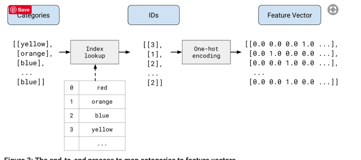
For each type of categorical data, each category has an integer code. In the figure above, each color has a code (0 for red, 1 for orange etc.) and they will eventually be transformed to the feature vector on the right, with vector length being the total number of categories found in the data, and the element will be filled with 1 if it is of that category. This allows a natural way of dealing with missing data (with all elements 0) and multi-category (with multiple non-zeros).

In natural language processing, the bag-of-words model is often used to represent free-text data, which is the one-hot encoding above with words as the categories. It is a good way as long as the order of the words does not matter.

Binary Data

For binary data, it can be easily represented by one element, either 1 or 0.

Graphical Data

Graphical data are best represented in terms of graph Laplacian and adjacency matrix. Refer to a previous blog article for more information.

Shortcomings

A feature vector can be a concatenation of various features in terms of all these types except graphical data.

However, such representation that concatenates all the categorical, binary, and numerical fields has a lot of shortcomings:

1. Data with different categories are often seen as orthogonal, i.e., perfectly dissimilar.  It ignores the correlation between different variables. However, it is a very big assumption.
2. The weights of different fields are not considered.
3. Sometimes if the numerical values are very large, it outweighs other categorical data in terms of influence in computation.
4. Data are very sparse, costing a lot of memory waste and computing time.
5. It is unknown whether some of the data are irrelevant.

Modifying Feature Vectors

In light of the shortcomings, to modify the feature factors, there are three main ways of dealing with this:

1. Rescaling: rescaling all of some of the elements, or reweighing, to adjust the influence from different variables.
2. Embedding: condensing the information into vectors of smaller lengths.
3. Sparse coding: deliberately extend the vectors to a larger length.

Rescaling

Rescaling means rescaling all or some of the elements in the vectors. Usually there are two ways:

1. Normalization: normalizing all the categories of one feature to having the sum of 1.
2. Term frequency-inverse document frequency (tf-idf): weighing the elements so that the weights are heavier if the frequency is higher and it appears in relatively few documents or class labels.

Embedding

Embedding means condensing a sparse vector to a smaller vector. Many sparse elements disappear and information is encoded inside the elements. There are rich amount of work on this.

1. Topic models: finding the topic models (latent Dirichlet allocation (LDA),  structural topic models (STM) etc.) and encode the vectors with topics instead;
2. Global dimensionality reduction algorithms: reducing the dimensions by retaining the principal components of the vectors of all the data, e.g., principal component analysis (PCA), independent component analysis (ICA), multi-dimensional scaling (MDS) etc;
3. Local dimensionality reduction algorithms: same as the global, but these are good for finding local patterns, where examples include t-Distributed Stochastic Neighbor Embedding (tSNE) and Uniform Manifold Approximation and Projection (UMAP);
4. Representation learned from deep neural networks: embeddings learned from encoding using neural networks, such as auto-encoders, Word2Vec, FastText, BERT etc.
5. Mixture Models: Gaussian mixture models (GMM), Dirichlet multinomial mixture (DMM) etc.
6. Others: Tensor decomposition (Schmidt decomposition, Jennrich algorithm etc.), GloVe etc.

Sparse Coding

Sparse coding is good for finding basis vectors for dense vectors.

Computational Folkloristics: Major Emotional Arcs for Good-Selling Fictions

The emotional flows of stories are important to engage the readers. Skillful writers grasp this very well by natural instinct. There are theories about this, called folkloristics. However, is there a way to see the flows in a graph? Linear algebra and natural language processing (NLP) kick in.

Andrew Reagan at the Computational Story Lab, University of Vermont, together with his colleagues and collaborators, did a numerical studies about this. [Reagan et. al., 2016] Their paper is now on the arXiv. He prepared a set of words with scores that quantitatively describe their sentiments, as in sentiment analysis. He then went through the text with a sliding window to measure the sentiments. Then for each book, there is a vector of a time series of these sentiment scores. For example, using this method, the plot of the emotional scores, or the emotional arc, of J. K. Rowling’s Harry Potter and the Deathly Hallows is as shown in the following plot: [Reagan et. al., 2016]

They did the same thing with other English fictions in the Project Gutenberg Corpus, giving a vector of these emotional scores for each fiction. They performed a principal component analysis (PCA) for all these books (represented by a matrix containing all vectors). PCA is a common dimensionality reduction techniques, and also useful for information retrieval (IR) in another name called latent semantic analysis (LSA). Reagan and his colleagues identify six major components of these emotional arcs, as shown below: [Reagan et. al., 2016]

These computational studies on fictions further reinforce our common belief that (good-selling) fictions do have resonating themes to keep the readers.

Starting the Journey of Topological Data Analysis (TDA)

Topology has been around for centuries, but it did not catch the attention of many data analysts until recently. In an article published in Nature Scientific Reports, the authors demonstrated the power of topology in data analysis through examples including gene expression from breast rumors, voting data in the United States, and player performance data from the NBA. [Lum et. al. 2013]

As an introduction, they described topological methods “as a geometric approach to pattern or shape recognition within data.” It is true that in machine learning, we never care enough pattern recognition, but topology adds insights regarding the shapes of data that do not change with continuous deformation. For example, a circle and an ellipse have “the same topology.” The distances between data points are not as important as the shape. Traditional machine learning methods deal with feature vectors, distances, or classifications, but the topology of the data is usually discarded. Gunnar Carlsson demonstrated in a blog that a thin ellipse of data may be misrepresented as two straight parallel lines or one straight lines. [Carlsson 2015] Dimensionality reduction algorithms such as principal component analysis (PCA) often disregard the topology as well. (I heard that Kohenen’s self-organizing maps (SOM) [Kohonen 2000] retain the topology of higher dimensional data during the dimensionality reduction, but I am not confident enough to say that.)

Euler introduced the concept of topology in the 18th century. Topology has been a big subject in physics since 1950s. The string theory, as one of the many efforts in unifying gravity and other three fundamental forces, employs topological dimensions. In condensed matter physics, the fractional quantum Hall effect is a topological quantum effect. There are topological solitons [Rajaraman 1987] such as quantum vortices in superfluids, [Simula, Blakie 2006; Calzetta, Ho, Hu 2010] columns of topological solitons (believed to be Skyrmions) in helical magnets, [Mühlbauer et. al. 2009; Ho et. al. 2010; Ho 2012] hexagonal solitonic objects in smectic liquid crystals [Matsumoto et. al. 2009]… When a field becomes sophisticated, it becomes quantitative; when a quantitative field becomes sophisticated, it requires abstract mathematics such as topology for a general description. I believe analysis on any kinds of data is no exception.

There are some good reviews and readings about topological data analysis (TDA) out there, for example, the ones by Gunnar Carlsson [Carlsson 2009] and Afra Zomorodian [Zomorodian 2011]. While physicists talk about homotopy, data analysts talk about persistent homology as it is easier to compute. Data have to be described in a simplicial complex or a graph/network. Then the homology can be computed and represented in various ways such as barcodes. [Ghrist 2008] Then we extract insights about the data from it.

Topology has a steep learning curve. I am also a starter learning about this. This blog entry will not be the last talking about TDA. Therefore, I opened a new session called TDA for all of my blog entries about it. Let’s start the journey!

There is an R package called “TDA” that facilitates topological data analysis. [Fasy et. al. 2014] A taste of homology of a simplicial complex is also demonstrated in a Wolfram demo.

(Taken from TheGuardian)