Tensor Networks in Machine Learning: Part I

In 2019, Google published a new Python library called “tensornetwork” (arXiv:1905.01330) that facilitates the computation of… tensor networks. Tensor network is a tool from quantum many-body theory, widely used in condensed matter physics. There have been a lot of numerical packages for tensor computation, but this library takes it to the next level because of its distinctive framework.

What is a tensor network, though?

“A tensor network is a collection of tensors with indices connected according to a network pattern. It can be used to efficiently represent a many-body wave-function in an otherwise exponentially large Hilbert space.”

https://www.perimeterinstitute.ca/research/research-initiatives/tensor-networks-initiative

Renormalization Group (RG)

It is not until recently that tensor networks have its application in machine learning. As stated in a previous post, a mathematical connection between restricted Boltzmann machine (RBM) and variational renormalization group (RG) was drawn. (arXiv:1410.1831) It shedded light to the understanding of interpretability of deep learning, which has been criticized to be a black box. However, RBM is just a type of unsupervised machine learning, but how about others?

Seeing this, Schwab, one of the authors of the RG paper, and Stoudenmire did some work to realize the use of RG in machine learning. Stoudenmore is a physicist, and he made use of density matrix renormalization group (DMRG) that he is familiar with, and invented a supervised learning algorithm, which is later renamed tensor network machine learning (TNML). The training is adapted from the sweeping algorithm, the standard of DMRG, that combining bipartite site one-by-one, updating it, and decomposing into two site by studying its quantum entanglment (using singular value decomposition, or Schmidt decomposition).

Instead of bringing interpretability to deep learning, this work in fact opened a new path of new machine learning algorithms with known techniques.

What is RG?

Renormalization group (RG) is a formalism of “zooming out” in scale-invariant system, determining which terms to truncate in a model. It is an important formalism in high energy physics and statistical field theory. (See Ma’s book for reference.)

Density matrix renormalization group (RG) is a variational real-space numerical technique that look at collections of quantum bits (zoomed-out) as a block. It was invented by Steven White, and it is useful in studying strongly correlated electronic systems. (PRL 69 (19): 2863-2866 (1992)). However, the original DMRG paper is not very accessible, until it is rephrased using the tensor network notation (TNN), as shown in Schollwoeck’s article.

Is Tensor Network Related to Quantum Computing?

This is not an easy question to answer. Tensor networks come from quantum physics, but quantum physics is usually not directly leading to quantum computing. In fact, classical computing hardwares have a lot of quantum physics in it. A simple answer to this question is no, as the algorithm using tensor network is implemented in classical computers.

There have been a lot of publications on quantum machine learning lately. A classic book on this topic is written by Peter Wittek. The book covers topics on basic machine learning and quantum computing, and then quantum machine learning algorithms. There is a quantum counterpart of each of the common machine learning algorithms in the book. However, we know it would be much more useful if there are new algorithms exploiting the advantages of quantum computing. Tensor network is a natural choice as it builds on qubits, and the representations and operations are naturally quantum.

Next…

Tensor network is an interesting subject from both a theoretical and applicational perspective. In coming posts I will talk about its application on machine learning and a taste of codes.


  • Github: google/TensorNetwork. [Github] [RTFD]
  • Chase Roberts, Ashley Milsted, Martin Ganahl, Adam Zalcman, Bruce Fontaine, Yijian Zou, Jack Hidary, Guifre Vidal, Stefan Leichenauer, “TensorNetwork: A Library for Physics and Machine Learning,” arXiv:1905.01330 (2019). [arXiv]
  • “Google TensorNetwork Library Dramatically Accelerates ML & Physics Tasks,” Syncedreview. (2019) [Medium]
  • Chase Roberts, “Introducing TensorNetwork, an Open Source Library for Efficient Tensor Calculations,” Google AI Blog. (2019) [GoogleAIBlog]
  • “Tensor Networks and Density Matrix Renormalization Group,” Everything About Data Analytics. (2016) [WordPress]
  • P. Mehta, D. J. Schwab, “An exact mapping between the Variational Renormalization Group and Deep Learning,” arXiv:1410.3831 (2014). [arXiv]
  • Sheng-kang Ma, Modern Theory of Critical Phenomena, (New York, NY: Routledge, 2018). [Amazon]
  • S. R. White, “Density matrix formulation for quantum renormalization groups,” Phys. Rev. Lett. 69, 2863 (1992). [APS]
  • Ulrich Schollwoeck, “The density-matrix renormalization group,” Rev. Mod. Phys. 77, 259 (2005); arXiv:cond-mat/0409292. [arXiv]
  • Ulrich Schollwoeck, “The density-matrix renormalization group in the age of matrix product states,” Annals of Physics 326, 96 (2011); arXiv:1008.3477. [arXiv]
  • Peter Wittek, Quantum Machine Learning: What Quantum Computing Means to Data Mining (San Diego, CA: Academic Press, 2014). [Amazon] [PDF]
  • Jacob Biamonte, Peter Wittek, Nicola Pancotti, Patrick Rebentrost, Nathan Wiebe, Seth Lloyd, “Quantum Machine Learning,” Nature 549, 195-202 (2017). [Nature]
  • Tensor Networks: From Entangled Quantum Matter to Emergent Space Time, Perimeter Institute. [Perimeter]

Feature picture taken from Perimeter Institute.

Data Representation in Machine Learning

In implementing most of the machine learning algorithms, we represent each data point with a feature vector as the input. A vector is basically an array of numerics, or in physics, an object with magnitude and direction. How do we represent our business data in terms of a vector?

Primitive Feature Vector

Whether the data are measured observations, or images (pixels), free text, factors, or shapes, they can be categorized into four following types:

  1. Categorical data
  2. Binary data
  3. Numerical data
  4. Graphical data

The most primitive representation of a feature vector looks like this:

Screen Shot 2019-09-15 at 3.58.09 PM
A typical feature vector. (Source: https://www.researchgate.net/publication/318740904_Chat_Detection_in_an_Intelligent_Assistant_Combining_Task-oriented_and_Non-task-oriented_Spoken_Dialogue_Systems/figures?lo=1)

Numerical Data

Numerical data can be represented as individual elements above (like Tweet GRU, Query GRU), and I am not going to talk too much about it.

Categorical Data

However, for categorical data, how do we represent them? The first basic way is to use one-hot encoding:

Screen Shot 2019-09-15 at 4.02.51 PM
One-hot encoding of categorical data (Source: https://developers.google.com/machine-learning/data-prep/transform/transform-categorical)

For each type of categorical data, each category has an integer code. In the figure above, each color has a code (0 for red, 1 for orange etc.) and they will eventually be transformed to the feature vector on the right, with vector length being the total number of categories found in the data, and the element will be filled with 1 if it is of that category. This allows a natural way of dealing with missing data (with all elements 0) and multi-category (with multiple non-zeros).

In natural language processing, the bag-of-words model is often used to represent free-text data, which is the one-hot encoding above with words as the categories. It is a good way as long as the order of the words does not matter.

Binary Data

For binary data, it can be easily represented by one element, either 1 or 0.

Graphical Data

Graphical data are best represented in terms of graph Laplacian and adjacency matrix. Refer to a previous blog article for more information.

Shortcomings

A feature vector can be a concatenation of various features in terms of all these types except graphical data.

However, such representation that concatenates all the categorical, binary, and numerical fields has a lot of shortcomings:

  1. Data with different categories are often seen as orthogonal, i.e., perfectly dissimilar.  It ignores the correlation between different variables. However, it is a very big assumption.
  2. The weights of different fields are not considered.
  3. Sometimes if the numerical values are very large, it outweighs other categorical data in terms of influence in computation.
  4. Data are very sparse, costing a lot of memory waste and computing time.
  5. It is unknown whether some of the data are irrelevant.

Modifying Feature Vectors

In light of the shortcomings, to modify the feature factors, there are three main ways of dealing with this:

  1. Rescaling: rescaling all of some of the elements, or reweighing, to adjust the influence from different variables.
  2. Embedding: condensing the information into vectors of smaller lengths.
  3. Sparse coding: deliberately extend the vectors to a larger length.

Rescaling

Rescaling means rescaling all or some of the elements in the vectors. Usually there are two ways:

  1. Normalization: normalizing all the categories of one feature to having the sum of 1.
  2. Term frequency-inverse document frequency (tf-idf): weighing the elements so that the weights are heavier if the frequency is higher and it appears in relatively few documents or class labels.

Embedding

Embedding means condensing a sparse vector to a smaller vector. Many sparse elements disappear and information is encoded inside the elements. There are rich amount of work on this.

  1. Topic models: finding the topic models (latent Dirichlet allocation (LDA),  structural topic models (STM) etc.) and encode the vectors with topics instead;
  2. Global dimensionality reduction algorithms: reducing the dimensions by retaining the principal components of the vectors of all the data, e.g., principal component analysis (PCA), independent component analysis (ICA), multi-dimensional scaling (MDS) etc;
  3. Local dimensionality reduction algorithms: same as the global, but these are good for finding local patterns, where examples include t-Distributed Stochastic Neighbor Embedding (tSNE) and Uniform Manifold Approximation and Projection (UMAP);
  4. Representation learned from deep neural networks: embeddings learned from encoding using neural networks, such as auto-encoders, Word2Vec, FastText, BERT etc.
  5. Mixture Models: Gaussian mixture models (GMM), Dirichlet multinomial mixture (DMM) etc.
  6. Others: Tensor decomposition (Schmidt decomposition, Jennrich algorithm etc.), GloVe etc.

Sparse Coding

Sparse coding is good for finding basis vectors for dense vectors.

Continue reading “Data Representation in Machine Learning”

Graph Convolutional Neural Network (Part II)

In the previous post, the convolution of the graph Laplacian is defined in its graph Fourier space as outlined in the paper of Bruna et. al. (arXiv:1312.6203) However, the eigenmodes of the graph Laplacian are not ideal because it makes the bases to be graph-dependent. A lot of works were done in order to solve this problem, with the help of various special functions to express the filter functions. Examples include Chebyshev polynomials and Cayley transform.

ChebNet

Kipf and Welling proposed the ChebNet (arXiv:1609.02907) to approximate the filter using Chebyshev polynomial, using the result proved by Hammond et. al. (arXiv:0912.3848) With a convolutional layer g_{\theta} \circ x, instead of computing it directly by \Phi^T g_{\theta} \Phi x, it approximates the filter in terms of Chebyshev polynomial:

g_{\theta} (\Lambda) \approx \sum_{k=0}^K \theta_k T_k(\Lambda),

where T_k(x) are the Chebyshev polynomials. It has been proved by Hammond et. al. that by well truncating this representation, Chebyshev polynomials are very good to approximate the function. Then the convolution is:

g_{\theta} \circ x \approx \sum_{k=0}^K \theta_k T_k (\Lambda) x.

Here, \theta’s are the parameters to be trained. This fixed the bases of the representation, and it speeds up computation. The disadvantage is that eigenvalues are clusters in a few values with large gaps.

CayleyNet

The problem of ChebNet led to the work of Levie et. al., (arXiv:1705.07664) who proposed another approximation is used using Cayley transform. They made use of the Cayley function:

C(\lambda) = \frac{\lambda - i}{\lambda + i},

which is a bijective function from \mathbb{R}^+ to complex unit half-circle. Instead of Chebyshev polynomials, it approximates the filter as:

g(\lambda) = c_0 + \sum_{j=1}^r \left[ c_j C^j (h \lambda) + c_j^{\ast} C^{j \ast} (h \lambda) \right] ,

where c_0 is real and other c_j’s are generally complex, and h is a zoom parameter, and \lambda’s are the eigenvalues of the graph Laplacian. Tuning $h$ makes one find the best zoom that spread the top eigenvalues. c‘s are computed by training. This solves the problem of unfavorable clusters in ChebNet.

MotifNet

All previous works are undirected graph. How do we deal with directed graph with an asymmetric graph Laplacian? Benson, Gleich, Leskovec published an important work on Science in 2016 (arXiv:1612.08447) to address this problem. Their approach is reducing a directed graph to a higher order structure called network motifs. There are 13 network motifs. For each network motif, one can define an adjacency matrix for that motif by \mathcal{M}_k, with elements \mathcal{M}_{k, ij} being the number of motifs in the graph the the edge (i, j) that it belongs to.

f1-large

Then one computes 13 graph Laplacians from these 13 adjacency matrices. These graph Laplacians are symmetric, like those of undirected graphs. Then any filters can be approximated by the following multivariate matrix polynomial, as suggested by Monti, Otness, and Bronstein in their MotifNet paper (arXiv:1802.01572):

f_{\Theta} (\Delta_1, \dots, \Delta_k) = \sum_{j=0}^P \sum_{k_1, \dots, k_j \in {1, \ldots, K}} \theta_{\theta_1, \ldots, \theta_k} \Delta_{k_1}, \ldots, \Delta_{k_j} .

Applications of image processing, citation networks etc.

Continue reading “Graph Convolutional Neural Network (Part II)”

Graph Convolutional Neural Network (Part I)

Suggested by some friends, I have been reading graph convolutional neural network. This is not a recent interest, as I have been interested in some graph-related problems (as I developed the graphflow package) and topological data analysis (TDA, as I developed the mogutda package). Graph theory is not a new field as well, but it is interesting to see how it is being applied in deep learning, as a lot of real-world relational data can be expressed in terms of graphs. (Examples: word relations, organizational structure, genes, internet etc.) With the increasing attention to neo4j, we know graph is coming to be hot.

It would be helpful to review some basic graph theory:

  • A graph is represented by \mathcal{G} = (V, E), where V and E are the nodes (vertices) and edges respectively.
  • A graph can be directed or undirected. In graph convolutional neural network, they are undirected usually.
  • The adjacency matrix A describes how nodes are connected: A_{ij} = 1 if there is an edge connecting from node i to node j, and 0 otherwise. A is a symmetric matrix for an undirected graph.
  • The incidence matrix B is another way to describe how nodes are connected: B_{ij} = 1 if a node i is connected with edge j. This is useful for undirected graph.
  • The degree matrix D is a diagonal matrix, with elements D_{ii} denotes the number of neighbors for node i in undirected matrix.
  • The function acting on the nodes is called the filter.
  • The graph Laplacian, or Kirchhoff matrix, is defined by L = D - A, and the normalized graph Laplacian is \tilde{L} = I - D^{-\frac{1}{2}} A D^{-\frac{1}{2}}.

The graph Laplacian is the most important matrix in graph convolutional neural network. It is analogous to the Laplacian operator in Euclidean space, \nabla^2. The reader can easily verify this by constructing a graph of 2D lattice and compute the graph Laplacian matrix, and find that it is the same as the discretized Laplacian operator.

We can also get some insights from the Euclidean analogue. In physics, the solution to the Laplacian equation is harmonic: the basis of the solution can be described in the spectral/Fourier space, as:

\nabla^2 \psi = - \omega^2 \psi,

And \psi \propto e^{\pm i \omega x}. In graph convolutional neural network, as Bruna et. al. suggested in 2013, the graph is calculated in the graph Fourier space, instead of directly dealing with the Laplacian matrix in all layers of network.

On the other hand, we know that for the convolution

(f \circ g) (x) = \int dy f(x-y) g(y),

its Fourier transform is given by

\tilde{( f \circ g)} (\omega) = \tilde{f} (\omega) \tilde{g} (\omega).

In Fourier space, the convolution of two functions are just their products. Similarly, in graph convolutional neural network, convolutions can be computed in the Fourier space as the mere product of two filters in the Fourier space. More specifically, for finding the convolution of the filters f and g, with \Phi being the unitary eigenmatrix,

f \circ g = \Phi ((\Phi^T g) \circ (\Phi^T f)) = \Phi \textbf{diag}(g_1, g_2, \ldots, g_n) f.

However, such general description is basis-dependent, and it is still computationally expensive. More work has been proposed to smooth the representation, which will be covered in the upcoming blogs.

A side note, the readers can verify themselves that

\sum_{ij} A_{ij} | f_i - g_j |^2 = f \tilde{L} g

Continue reading “Graph Convolutional Neural Network (Part I)”

New Family of Regularization Methods

In their paper, Kawaguchi, Kaelbling, and Bengio explored the theory of why generalization in deep learning is so good. Based on their theoretical insights, they proposed a new regularization method, called Directly Approximately Regularizing Complexity (DARC), in addition to commonly used Lp-regularization and dropout methods.

This paper explains why deep learning can generalize well, despite large capacity and possible algorithmic instability, nonrobustness, and sharp minima, effectively addressing an open problem in the literature. Based on our theoretical insight, this paper also proposes a family of new regularization methods. Its simplest member was empirically shown to improve base models and achieve state-of-the-art performance on MNIST and CIFAR-10 benchmarks. Moreover, this paper presents both data-dependent and data-independent generalization guarantees with improved convergence rates. Our results suggest several new open areas of research.

Screen Shot 2017-10-24 at 11.41.41 PM

Continue reading “New Family of Regularization Methods”

Word Mover’s Distance as a Linear Programming Problem

Much about the use of word-embedding models such as Word2Vec and GloVe have been covered. However, how to measure the similarity between phrases or documents? One natural choice is the cosine similarity, as I have toyed with in a previous post. However, it smoothed out the influence of each word. Two years ago, a group in Washington University in St. Louis proposed the Word Mover’s Distance (WMD) in a PMLR paper that captures the relations between words, not simply by distance, but also the “transportation” from one phrase to another conveyed by each word. This Word Mover’s Distance (WMD) can be seen as a special case of Earth Mover’s Distance (EMD), or Wasserstein distance, the one people talked about in Wasserstein GAN. This is better than bag-of-words (BOW) model in a way that the word vectors capture the semantic similarities between words.

Word Mover’s Distance (WMD)

The formulation of WMD is beautiful. Consider the embedded word vectors \mathbf{X} \in R^{d \times n}, where d is the dimension of the embeddings, and n is the number of words. For each phrase, there is a normalized BOW vector d \in R^n, and d_i = \frac{c_i}{\sum_i c_i}, where i‘s denote the word tokens. The distance between words are the Euclidean distance of their embedded word vectors, denoted by c(i, j) = || \mathbf{x}_i - \mathbf{x}_j ||_2, where i and j denote word tokens. The document distance, which is WMD here, is defined by \sum_{i, j} \mathbf{T}_{i j} c(i, j), where \mathbf{T} is a n \times n matrix. Each element \mathbf{T}_{ij} \geq 0 denote how nuch of word i in the first document (denoted by \mathbf{d}) travels to word j in the new document (denoted by \mathbf{d}').

Then the problem becomes the minimization of the document distance, or the WMD, and is formulated as:

\text{min}_{\mathbf{T} \geq 0} \sum_{i, j=1}^n \mathbf{T}_{ij} c(i, j),

given the constraints:

\sum_{j=1}^n \mathbf{T}_{ij} = d_i, and

\sum_{i=1}^n \mathbf{T}_{ij} = d_j'.

This is essentially a simplified case of the Earth Mover’s distance (EMD), or the Wasserstein distance. (See the review by Gibbs and Su.)

Using PuLP

The WMD is essentially a linear optimization problem. There are many optimization packages on the market, and my stance is that, for those common ones, there are no packages that are superior than others. In my job, I happened to handle a missing data problem, in turn becoming a non-linear optimization problem with linear constraints, and I chose limSolve, after I shop around. But I actually like a lot of other packages too. For WMD problem, I first tried out cvxopt first, which should actually solve the exact same problem, but the indexing is hard to maintain. Because I am dealing with words, it is good to have a direct hash map, or a dictionary. I can use the Dictionary class in gensim. But I later found out I should use PuLP, as it allows indices with words as a hash map (dict in Python), and WMD is a linear programming problem, making PuLP is a perfect choice, considering code efficiency.

An example of using PuLP can be demonstrated by the British 1997 UG Exam, as in the first problem of this link, with the Jupyter Notebook demonstrating this.

Implementation of WMD using PuLP

The demonstration can be found in the Jupyter Notebook.

Load the necessary packages:

from itertools import product
from collections import defaultdict

import numpy as np
from scipy.spatial.distance import euclidean
import pulp
import gensim

Then define the functions the gives the BOW document vectors:

def tokens_to_fracdict(tokens):
    cntdict = defaultdict(lambda : 0)
    for token in tokens:
        cntdict[token] += 1
    totalcnt = sum(cntdict.values())
    return {token: float(cnt)/totalcnt for token, cnt in cntdict.items()}

Then implement the core calculation. Note that PuLP is actually a symbolic computing package. This function return a pulp.LpProblem class:

def word_mover_distance_probspec(first_sent_tokens, second_sent_tokens, wvmodel, lpFile=None):
    all_tokens = list(set(first_sent_tokens+second_sent_tokens))
    wordvecs = {token: wvmodel[token] for token in all_tokens}

    first_sent_buckets = tokens_to_fracdict(first_sent_tokens)
    second_sent_buckets = tokens_to_fracdict(second_sent_tokens)

    T = pulp.LpVariable.dicts('T_matrix', list(product(all_tokens, all_tokens)), lowBound=0)

    prob = pulp.LpProblem('WMD', sense=pulp.LpMinimize)
    prob += pulp.lpSum([T[token1, token2]*euclidean(wordvecs[token1], wordvecs[token2])
                        for token1, token2 in product(all_tokens, all_tokens)])
    for token2 in second_sent_buckets:
        prob += pulp.lpSum([T[token1, token2] for token1 in first_sent_buckets])==second_sent_buckets[token2]
    for token1 in first_sent_buckets:
        prob += pulp.lpSum([T[token1, token2] for token2 in second_sent_buckets])==first_sent_buckets[token1]

    if lpFile!=None:
        prob.writeLP(lpFile)

    prob.solve()

    return prob

To extract the value, just run pulp.value(prob.objective)

We use Google Word2Vec. Refer the \mathbf{T} matrices in the Jupyter Notebook. Running this by a few examples:

  1. document1 = President, talk, Chicago
    document2 = President, speech, Illinois
    WMD = 2.88587622936
  2. document1 = physician, assistant
    document2 = doctor
    WMD = 2.8760048151
  3. document1 = physician, assistant
    document2 = doctor, assistant
    WMD = 1.00465738773
    (compare with example 2!)
  4. document1 = doctors, assistant
    document2 = doctor, assistant
    WMD = 1.02825379372
    (compare with example 3!)
  5. document1 = doctor, assistant
    document2 = doctor, assistant
    WMD = 0.0
    (totally identical; compare with example 3!)

There are more examples in the notebook.

Conclusion

WMD is a good metric comparing two documents or sentences, by capturing the semantic meanings of the words. It is more powerful than BOW model as it captures the meaning similarities; it is more powerful than the cosine distance between average word vectors, as the transfer of meaning using words from one document to another is considered. But it is not immune to the problem of misspelling.

This algorithm works well for short texts. However, when the documents become large, this formulation will be computationally expensive. The author actually suggested a few modifications, such as the removal of constraints, and word centroid distances.

Example codes can be found in my Github repository: stephenhky/PyWMD.

Continue reading “Word Mover’s Distance as a Linear Programming Problem”

“selu” Activation Function and 93 Pages of Appendix

A preprint on arXiv recently caught a lot of attentions. While deep learning is successful in various types of neural networks, it had not been so for feed-forward neural networks. The authors of this paper proposed normalizing the network with a new activation function, called “selu” (scaled exponential linear units):

\text{selu}(x) =\lambda \left\{ \begin{array}{cc} x & \text{if } x>0  \\ \alpha e^x - \alpha & \text{if } x \leq 0  \end{array}  \right..

which is an improvement to the existing “elu” function.

Despite this achievement, what caught the eyeballs is not the activation function, but the 93-page appendix of mathematical proof:

lol

And this is one of the pages in the appendix:

longproof

Some scholars teased at it on Twitter too:

Continue reading ““selu” Activation Function and 93 Pages of Appendix”

On Wasserstein GAN

A few weeks ago, I introduced the generative model called generative adversarial networks (GAN), and stated the difficulties of training it. Not long after the post, a group of scientists from Facebook and Courant introduced Wasserstein GAN, which uses Wasserstein distance, or the Earth Mover (EM) distance, instead of Jensen-Shannon (JS) divergence as the final cost function.

In their paper (arXiv:1701.07875), they proposed the following to improve GAN:

  • do not use sigmoid function as the activation function;
  • the cost functions of the discriminator and generator must not have logarithms;
  • cap the parameters at each step of training; and
  • do not use momentum-based optimizer such as momentum or Adam; instead, RMSprop or SGD are recommended.

These do not have a theoretical reason, but rather empirical. However, the most important change is to use the Wasserstein distance as the cost function, which the authors explained in detail. There are many metrics to measure the differences between probability distributions, as summarized by Gibbs and Su in the paper, (arXiv:math/0209021) the authors of Wasserstein GAN discussed four of them, namely, the total variation (TV) distance, the Kullback-Leibler (KL) divergence, the Jensen-Shannon (JS) divergence, and the Earth-Mover (EM, Wasserstein) distance. They used an example of two parallel uniform distributions in a line to illustrate that only the EM (or Wasserstein) distance captured the continuity of the distribution distances, solving the problem of zero-change when the derivative of the generator becoming too small. The EM distance indicates, intuitively, how much “mass” must be transported from one distribution to another.

Formally, the EM distance is

W(\mathbb{P}_r, \mathbb{P}_g) = \inf_{\gamma \in (\mathbb{P}_r, \mathbb{P}_g)} \mathbb{E}_{(x, y) \sim \gamma} [ || x-y||],

and the training involves finding the optimal transport path \gamma.

Unfortunately, the EM distance cannot be computed directly from the definition. However, as an optimization problem, there is a dual problem corresponding to this. While the author did not explain too much, Vincent Herrmann explained about the dual problem in detail in his blog.

The algorithm is described as follow:

v2-6be6e2ef3d15c4b10c2a943e9bf4db70_r

Continue reading “On Wasserstein GAN”

Generative Adversarial Networks

Recently I have been drawn to generative models, such as LDA (latent Dirichlet allocation) and other topic models. In deep learning, there are a few examples, such as FVBN (fully visible belief networks), VAE (variational autoencoder), RBM (restricted Boltzmann machine) etc. Recently I have been reading about GAN (generative adversarial networks), first published by Ian Goodfellow and his colleagues and collaborators. Goodfellow published his talk in NIPS 2016 on arXiv recently.

Yesterday I attended an event at George Mason University organized by Data Science DC Meetup Group. Jennifer Sleeman talked about GAN. It was a very good talk.

In GAN, there are two important functions, namely, the discriminator (D), and the generator (G). As a generative model, the distribution of training data, all labeled positive, can be thought of the distribution that the generator was trained to produce. The discriminator discriminates the data with positive labels and those with negative labels. Then the generator tries to generate data, probably from noises, which should be negative, to fake the discriminator to see it as positive. This process repeats iteratively, and eventually the generator is trained to produce data that are close to the distribution of the training data, and the discriminator will be confused to classify the generated data as positive with probability \frac{1}{2}
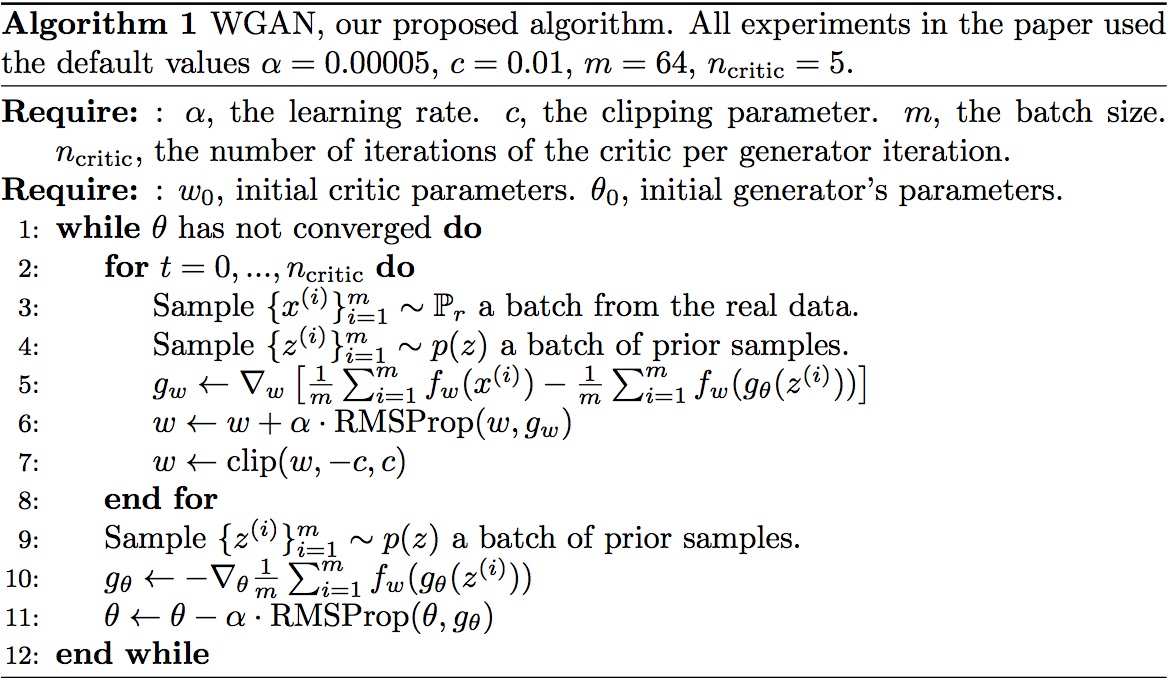
. The intuition of this competitive game is from minimax game in game theory. The formal algorithm is described in the original paper as follow:
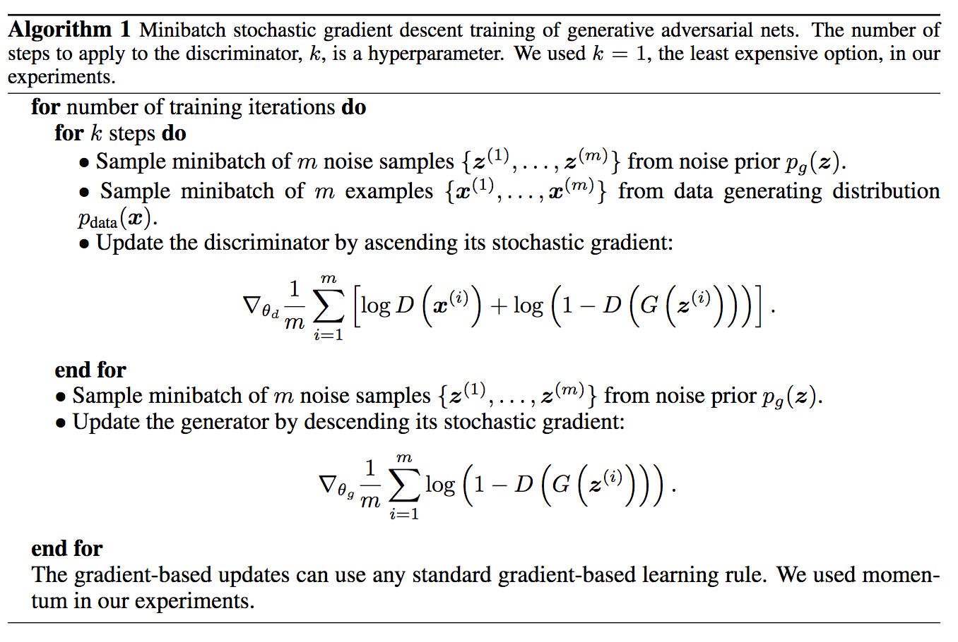
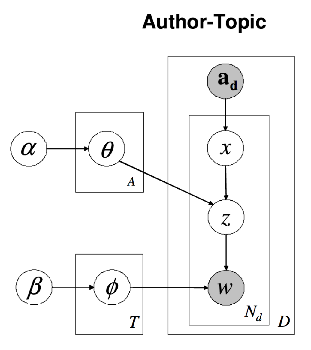
gan_algorithm

The original paper discussed about that the distribution of final generated data identical to that of the training data being the optimal for the model, and argued using the Jensen-Shannon (JS) divergence. Ferenc Huszár discussed in his blog about the relations between maximum likelihood, Kullback-Leibler (KL) divergence, and Jensen-Shannon (JS) divergence.

I have asked the speaker a few questions about the concepts of GAN as well.

GAN is not yet a very sophisticated framework, but it already found a few industrial use. Some of its descendants include LapGAN (Laplacian GAN), and DCGAN (deep convolutional GAN). Applications include voice generation, image super-resolution, pix2pix (image-to-image translation), text-to-image synthesis, iGAN (interactive GAN) etc.

Adversarial training is the coolest thing since sliced bread.” – Yann LeCun

16427477_10105464843466738_3344635019272539994_n


Continue reading “Generative Adversarial Networks”

Author-Topic Models in gensim

Recently, gensim, a Python package for topic modeling, released a new version of its package which includes the implementation of author-topic models.

The most famous topic model is undoubtedly latent Dirichlet allocation (LDA), as proposed by David Blei and his colleagues. Such a topic model is a generative model, described by the following directed graphical models:

lda_pic

In the graph, \alpha and \beta are hyperparameters. \theta is the topic distribution of a document, z 
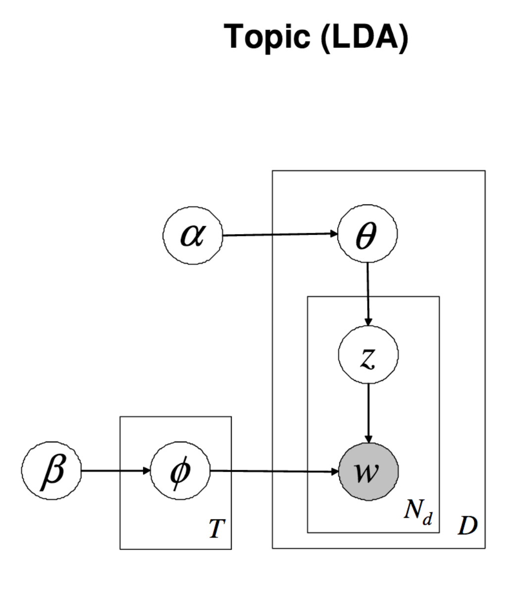
is the topic for each word in each document, \phi is the word distributions for each topic, and w is the generated word for a place in a document.

There are models similar to LDA, such as correlated topic models (CTM), where \phi is generated by not only \beta but also a covariance matrix \Sigma.

There exists an author model, which is a simpler topic model. The difference is that the words in the document are generated from the author for each document, as in the following graphical model. x is the author of a given word in the document.
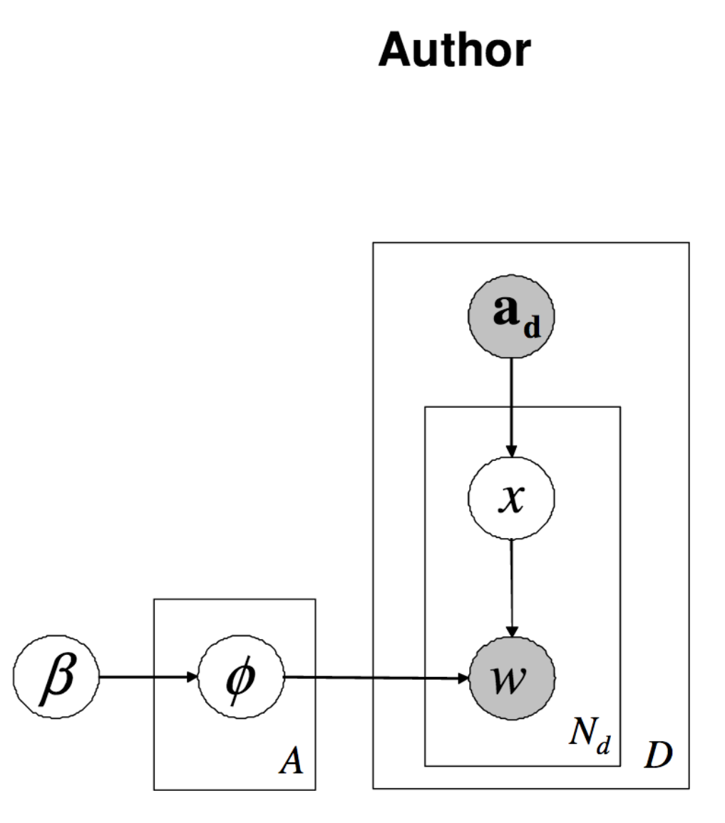
author_pic

Combining these two, it gives the author-topic model as a hybrid, as shown below:

authortopic_pic

The new release of Python package, gensim, supported the author-topic model, as demonstrated in this Jupyter Notebook.

P.S.:

  • I am also aware that there is another topic model called structural topic model (STM), developed for the field of social science. However, there is no Python package supporting this, but an R package, called stm, is available for it. You can refer to their homepage too.
  • I may consider including author-topic model and STM in the next release of the Python package shorttext.

Continue reading “Author-Topic Models in gensim”

Create a free website or blog at WordPress.com.

Up ↑